Pathway Logic Assistant Reference Guide
The Pathway Logic Assistant (PLA) allows you to explore a Pathway logic knowledge base (KB) and to query models derived from such a KB. One interacts with PLA via two main types of window: the knowledge base manager (KBManager, unique to a session) and graph viewer windows (zero or more per session). A model can be derived using a predefined initial state (called a dish), or by interactively creating an initial state using the dish editor. Dishes represent the cell state in a hypthetial experimental setup. The resulting model is represented as a Petri net whose transitions are the KB rules reachable from the initial state. The Petri net graph is displayed in the PLA viewer which the user can use to browse the network and query the model for subnets and pathways. Using PLA you can also incrementally explore the KB network by specifying a set of rules or occurrences from which to start and then selectively adding connected rules and occurrences. In addition, graphs (i.e. the underlying networks) that have been constructed by querying models or exploring can be compared. A graph viewer has a mode determined by the interface provided by the underlying network: Pnet for networks generated from a dish (models) and subnets resulting from queries; Xnet for networks generated by exploring; and Cnet for comparison nets. The reason for modes is that the meaningful operations/interactions depend on the mode (how the network was generated).
KBManager Window
  Creating a Model
    Dish Editor
  Exploring a Network
    From Occs
    From Rules

PLA Graph Viewer
  Using Tabs
  Navigation
  Information
  Menus
  ToolBar

Mode Specific Functionality
  Pnet
  Xnet
  Cnet
KBManager Window
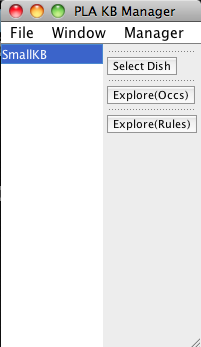
When PLA starts up it loads a knowledge base (KB) and displays a knowledge base manager window (title: PLA KBManager) in the upper left corner of your screen. The KBManager displays a list of available knowledge bases (rule sets). Initially, there is just one KB. The currently selected KB highlighted in blue.
The KBManager has three buttons on the right. Use one of these buttons to open a PLA viewer window displaying the corresponding network graph.
- Select Dish --- create a model to study.
- Explore(Occs) --- explore the KB starting with occurrences chosen from a list of known occurrences.
- Explore(Rules) --- explore the KB starting with rules chosen from a list of rules in the KB.
Creating a Model
To create a model press the "Select Dish" button. You will be offered two choices, "edit" and "predefined", from a drop down menu. If you select "predefined", a list of available dishes will be displayed. Click on one of the listed dishes to select it. If you select edit, a dish editor dialog will open. Use this to specify a dish (see below). In either case, once you have specified a dish PLA will display the resulting model (a Pnet) in a graph viewer window in Pnet mode. You can use the viewer to browse and analyze the model (see the section on the graph viewer).
If you select "Edit", a dish editor dialogue will appear which you can use to create an initial state (aka dish). The dish editor has two columns: the left column (labeled Dish) lists the set of occurrences currently in your dish; the right column (labeled Scope) lists the set of occurrences from which you can choose. The occurrence lists are grouped into sublist according to the first character of the occurrence name. As shown is the leftmost dish editor screen shot below, initially the Dish column is empty and the Scope column contains all the occurrences that appear in the KB.
|
Dish Editor: before editing |
Dish Editor with Egf-Out, EgfR-CLm, Gab1-CLc, Gab2-CLc, and Sos1-CLc checked |
Dish Editor after pressing the "Add" button. Egf-Out, EgfR-CLm, Gab1-CLc, and Gab2-CLc are now in the dish. |
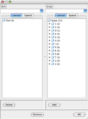
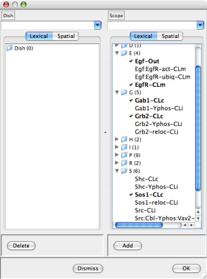
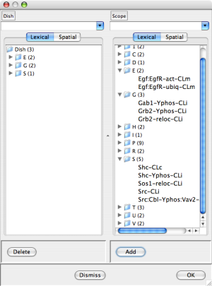
You can add occurrences to the dish by selecting them from the scope (checking the associated box) and pressing the "Add" button at the bottom of the Scope column. Dually, you can remove occurrences from the dish by checking the associated boxes and pressing the "Delete" button at the bottom of the Dish column. In more detail click on the triangle to the left of a sublist to expose the sublist items for selection. The center dish editor screen shot above shows a dish dialog after checking Egf-Out, EgfR-CLm, Gab1-CLc, Gab2-CLc, and Sos1-CLc. The rightmost dish editor screen shot above shows the result of pressing the "Add" button. Notice that the selected occurrences have disappeared from the Scope and non-empty sublists in the E,G, and S categories have appeared in the Dish.
The pair of buttons at the top of the Dish and Scope lists control the grouping of occurrences into sublists (categorization). The "Lexical" button selects lexical grouping according to the first character (the initial setting). The "Spatial" button groups occurrences according to lacation. (Try it.)
You can also select an occurrence by typing the first few characters. Matching occurrences will appear in a drop down list from which to select.
Using the Dish menu at the top of the Dish column you can save your
dish in a file, load a saved dish from a file, or load a predefined dish. In
the case of loading or saving a dish, a file chooser dialog will appear
to allow you specify the file name.
In the case of a predefined dish, you will be shown a list of
available dishes to choose from. Thus, using the dish editor you can define
variations on a basic dish, for example adding different ligands, or combine
dishes. At any point you can exit the dish Editor by
pressing the "Dismiss" button at the bottom of the window. Once you have created
a dish/initial state you want to study,
press the "OK" button at the bottom of the window.
An input dialog will appear asking for a name for the new dish. Type in a name
(please no spaces or other non-printing characters)
and press
Exploration of a KB can be initialized by selecting
a starting set of occurrences or a starting set of rules.
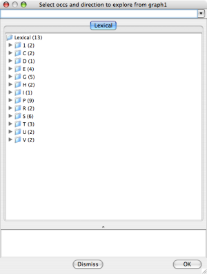
To explore a KB network starting with a given set of occurrences
click Explore(Occs). A selection dialog (titled Select occs and direction to
explore from < graph id >) will appear. The occurrences to select from
(all that appear connected to a rule in the KB) are grouped according to
the first letter of their label.
The leftmost selection dialog screen shot below shows the initial
dialog state. Click on the triangle pointing
to a letter to expose the occurrences in that group. For example
the E group of the SmallKB contains 4 occurrences:
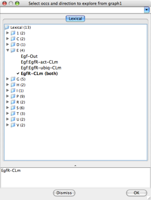
An occurrence can be selected for exploration up, down, or both.
The first click on an occurrence selects it for both. Repeated
clicking cycles through the options: both, up, down, (not selected).
The rightmost selection dialog screen shot below shows the result
of selecting EgfR-CLm for both.
If you click on
the folder icon, you will be given the option to select all items
in the list, none of the items, or reverse the current selection.
Explore Occurrences |
Explore Occurrences |
A list of selected occurrences appears in the pane at the bottom of the dialog, for convenience.
At any point, pressing the "Dismiss" button will cancel the Explore request. When you are finished choosing occurrences and their exploration directions, press the "OK" button on the bottom right. Shortly an Xnet graph view window (Xnet mode) will appear with the graph of the network formed from the selected occurrences and associated rules. If the "up" option is specified for an occurrence, the associated rules are those rules whose output includes that occurrence (upstream rules). If the "down" option is specified for an occurrence, the associated rules are those rules whose input (reactants and modifiers) includes that occurrence (downstream rules). The "both" option corresponds to the union of the up and down rules. Note that when a rule is included in a network, all of its connected occurrences are included as well.
To explore a KB network starting with a given set of rules press Explore(Rules). A selection dialog (titled: Select rules to add to < graph id >>) will appear. The rules to select from (all rules in the KB) are grouped according to the first character their label. Rule selection works like occurrence selection except there is no direction option. At any time you may press the "Dismiss" button to exit the selection dialog without submitting an Explore request. When you are finished selecting rules, press the "OK" button on the bottom right. Shortly an Xnet graph view window (Xnet mode) will appear with the graph of the network containing the selected rules.
PLA Graph Viewer
The PLA Graph Viewer uses tab frames and a graph hierarchy to organize windows.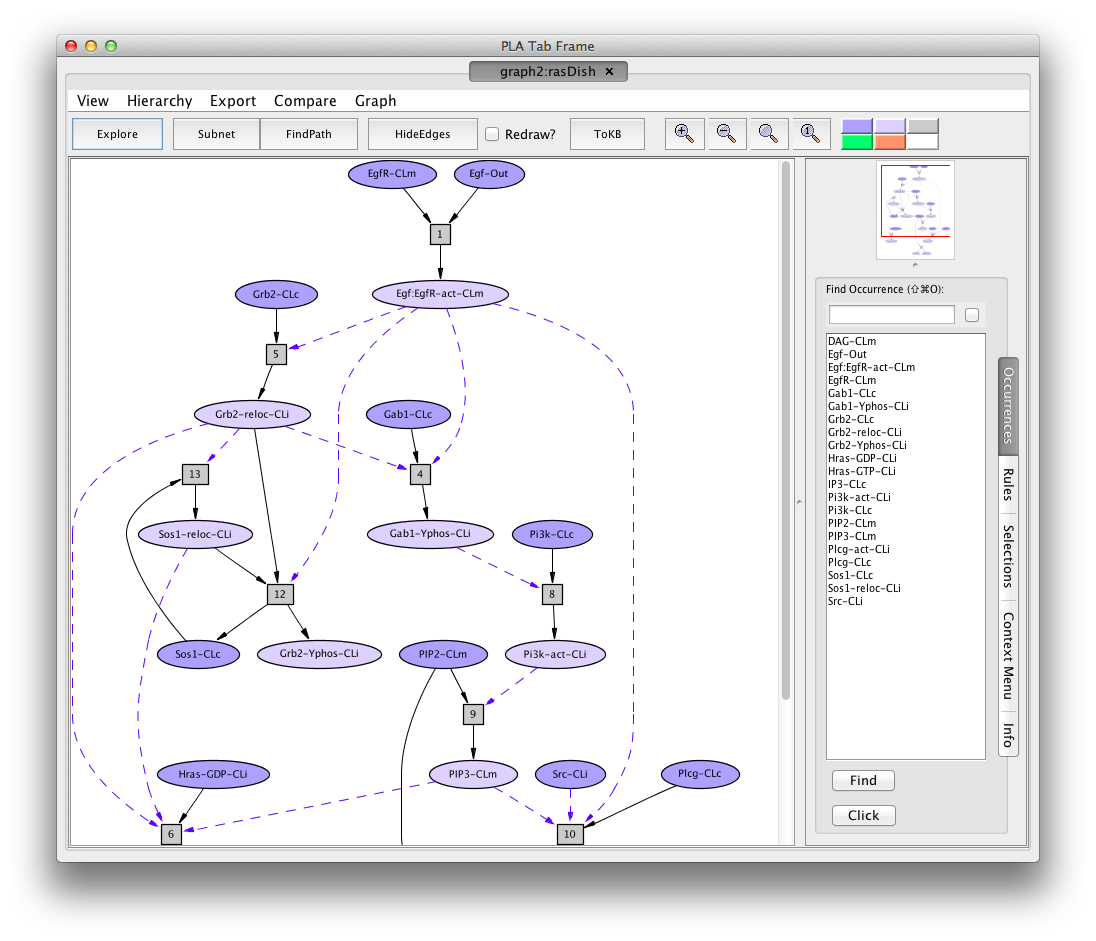
Screen shot of the Hras dish graph
- Title: the tab label. It tells you the graph identifier,and how the graph was constructed. The latter is either a dishnet described by the dish name, a subnet S(graphid), a pathnet P(graphid), an explorenet E(graphid), or a comparison C(source-graph,target-graph).
- Menu and Tool bars: the top and second rows of buttons
- Graph and navigation panels: left and right under the toolbar
- Information panel: bottom right. The information panel has five tabs: Occurrences,Rules, Selections, and Context and Info. By default the Occurrences tab is open. The other tabs can be opened (if available) by clicking on the tab name.
The menus and toolbar functions, and the information tabs will be explained below. The navigation panel displays a thumb nail sketch of the full graph with a red rectangle indicating the part of the graph visible in the graph panel.
In the graph panel, the network of reactions is displayed as a graph with two kinds of node, occurrence and rule. Ovals represent occurrences---proteins or chemicals in a specific state and location. For example the oval labelled EgfR-act-CLm represents an Efg receptor (also known as ErBb1) that is activated (-act) and located in the cell membrane (-CLm). We use the following abbreviations here.
Locations
  Out --- outside the cell, the medium or supernatant
  CLm --- in/across the cell membrane
  CLi --- attached to the inside of the cell membrane
  CLc --- in the cytoplasm

Modifications
 Yphos --- phosphorylated on a tyrosine
 act   --- activated
 reloc --- relocated
 ubiq  --- ubiquitinated
 GDP   --- loaded with Guanosine diphosphate (GDP)
 GTP   --- loaded with Guanosine triphosphate (GTP)
Darker colored ovals represent occurrences in the initial state (the selected dish when the network is generated by selected a dish). Lighter colored ovals represent potenial states/locations of these components. Rectangles represent reaction rules. The label in a reactangle is its (abbreviated) identifier in the knowledge base. Solid arrows from an occurrence oval to a rule indicate that the occurrence is a reactant (rule input). Solid arrows from a rule to an occurrence oval indicate that the occurrence is a product (rule output). Dashed arrows from an occurrence oval to a rule indicate that the occurrence is a modifier/enzyme/control. It is necessary for the reaction to take place but is not changed by the reaction.
As mentioned earlier there are three types of graph---Pnet, Xnet, and Cnet---depending on how the graph was generated:
- Pnet graphs are graphs of models, and subnets derived by queries. They have an initial state.
- Xnet graphs are graphs generated by exploration
- Cnet graphs are generated by graph comparison.
The graph viewer mode (Pnet, Xnet, or Cnet) reflects the graph type. The available functionality in the menu and tool bars and the information pane depend on the graph type, according to what is meaningful for the type.
We begin by describing the network-type independent features.
Using Tabs
Each new dishnet graph is displayed in a new tab frame (a new window). A child
graph, created as a subnet, pathnet or explorenet from a graph, is displayed as
a new tab in the parent's tab frame. Any tab in a multitab frame can be
displayed in a new frame by dragging it onto the desktop (hover your mouse over
the left end of the tab, a square will light up, grab and drag). The gripper
can also be used to drag a tab from one frame to another, or to reorder tabs in
a frame.
-
You can change the portion of the graph shown in the graph panel using the
thumbnail in two ways
- click on a spot in the thumbnail to center the graph view on that point
- drag the red rectangle to change the region shown in the graph view
-
Using the Occurrences tab in the information pane, you can bring a specific
occurrence into the graph view port. Open the tab by clicking on the tab name
(if it is not already open) and select the desired occurrence. There are two
ways find an occurrence: use the scroll bar at the side of the column to bring
the name/label into view; or type the first few letters of the name into the
text box at the top of the column. In this case the first matching name will
come into view, hilited in gray. Press
to cycle through the matching names. Click on a name to select it (the name will be highlited). Now there are three ways to bring the selected item into view in the graph panel.
- double click on the selected item (you can do this rather than single click to select in the first place)
- press Find at the bottom of the column
- press Click at the bottom of the column (This has the same effect as pressing Find and then clicking on the item in the graph panel.)
In all three cases the graph view will be centered on the selected occurrence and the border of item will become red to make it easy to see. In the case of pressing Click, the Context menu for the selected item will be displayed in the informantion panel (see #nodeInfo). Bringing a rule node into the view pane works the same way, using the Rules information tab.
-
To find what is at the other end of an arrow (edge), click on the arrow
and the Context Menu for the arrow will appear in the information panel.
The title tells you then name of the node at the other end, and there
are three buttons providing different action options.
- Goto the node at the other end (off screen)
- Center on the visible end
- Center on the other end
Press one of the buttons to perform the indicated reaction. You can also double click on the arrow to directly go to the other end (bring the other end into the viewport).
Information (Context Menu Tab)
You can obtain general information about the graph, a node, or an edge in the Context Menu tab of the Information pane.
- Clicking anywhere in the background of the graph pane will display a term describing how the graph was constructed in the information pane. The term has the form op[parent,args]. Here op indicates the function such as dishNet, subnet, pathnet, compare or explore. Parent is the identifier of the graph or knowledgebase from which the operation was invoked. Args depends on the operation. For a dishNet, the argument is the dishname. For a subnet or pathnet the arguments are the goals, avoids, and hidden rules. For exploring the arguments are the sequence of exploration operations, For comparison, the argument is the name of the graph that the parent is being compared to. The intent is that the graph can be reproduced using this term.
-
The graph context menu can be accessed from the Graph menu, or
by the keyboard shortcut
I. The information consists of internal information about the graph, and is mostly useful to PLA developers. - Clicking on the background of the graph pane in any tab will display the graph identifier and description for ???
-
A node context menu can be accessed by clicking on the node
(or by using the Occurrences or Rules and the Click button).
-
An occurrence context menu shows the full name of the occurrence
at the top. There are two `information' buttons and possibly
additional mode dependent options (see discussion of
mode specific functionality).
- The Show Info button displays internal information about the occurrence. This information is mostly useful for PLA developers.
- The About Occurrence button provides information about the base entity of the occurrence. What is displayed is be specified by the model developer. For proteins this typically includes the HUGO name, a link to the SwissProt page, synonyms, and possibly other links. For chemicals the metadata may include a link to the KEGG or PubChem entry for the chemical, where much information can be found along with links to other sources.
-
A rule context menu shows the full rule identifier at the top. There are
three `information' buttons and possibly additional mode dependent options
(see discussion of modes).
- The Show Info button displays internal information about the rule. This information is mostly useful for PLA developers.
- The show Maude Rule button displays the rewrite rule underlying the Petri net rule in Maude syntax. Mostly useful to model developers.
- The Show Evidence button displays evidence items provided by the rule curator. This may be just a list of pubmed links to papers used in curating the rule, or the set of evidence items curated from the papers, depending on how the model was developed.
The Explore Rule button is equivalent using the Explore Toolbar button
and selecting this rule as the single rule to explore from.
The main purpose is to allows you to see the Petri net graph of the rule
in isolation, and hence nicely formatted. You can continue
exploring at this point if you like.
-
An occurrence context menu shows the full name of the occurrence
at the top. There are two `information' buttons and possibly
additional mode dependent options (see discussion of
mode specific functionality).
- Context menus for graph edges are purely for navigation and are the same in all graphs (see #navigation-edges).
There are four mode independent menus: File, View, Hierearchy, Export, Compare, and Graph. They appear in that order (left to right) just under the tab.
The View Menu shows the top level frames (also known as windows) and the graphs they contain, as well as the KB Manager frame/window. Clicking on one ot the elements will bring it to the front.
The Hierarchy Menu shows the graph hiereary, independent of the windows. Again, clicking on a graph will bring it to the front. If you have closed a tab, the graph that was in that tab will show in red, and clicking on it will launch a new tab displaying the graph.
The Export Menu contains the following items
-
Export Image (shortcut
e) --- use this to save an image of the graph in Extended Postscript (eps), Portable Network Graphics (png), Dot (xdot), or Scalable Vector Graphics (svg) format. -
Export Graph (shortcut
g) --- use this to save the graph in one of several text formats that can be read by different tools. Currently available .lsp (read by JLambda for navigatable display), .sbml (Systems Biology Markup Language), .pn (an easily parsable description of the Petri net). This menu item is not currently available from the server.
The Compare Menu provides access to the graph comparison functionality. The current graph can be compared to any visible graph (other than its self) by selecting (clicking on) this menu and choosing one of the graphs presented. When you select the Compare menu, the visible graph names are displayed using the window hierarchy organization (see #WindowMenu), allowing you to readily see the relationships amongst the available graphs. The current graph will be grey (non selectable).
Once you have selected a "compare to" graph, the comparison graph (a Cnet) will be displayed in a new window (CNet mode). The comparison graph is simply the union of the nodes of the two graphs being compared. Nodes in both graphs a colored pink, nodes in the requesting graph are colored blue/lavendar, and nodes in the compare to graph are cyan (blue-green).
Note that comparing a graph to its parent is visually similar to viewing the graph in context, although comparing creates a new graph that you can manipulate, while viewing in context just draws it differently.
The Graph Menu provides a way to customize the graph's display, and to obtain information about the graph.
Every PLA graph view window has at least the following buttons in its tool bar (right to left)
- Color Key
- Zoomies (4)
- InContext/DotLayout (if the graph has a parent graph)
- ToKB
Color Key: The color of a graph node is used to convey status information. Place the mouse pointer over a color rectangle and a little text box (tooltip) will appear with a brief description of the meaning of the color. The colors used and their meaning depends on the mode. When the graph is rendered "InContext" (see #InContext/DotLayout) context nodes are white. Mode specific colors are explained in the discussion of each mode.
Zoomies: There are four zoomies (magnifying glass icons) each labeled with an indicator of the functionality. The zoomies can be used to resize the graph panel viesw of the graph.
- + (Zoom in): you see less of the graph, but the elements are larger.
- - (Zoom out): the opposite of Zoome in.
-
(Zoom to fit): fit the full graph inside the graph panel - 1 (Original size): reset the size to the original.
InContext/DotLayout: This button only appears if the graph has a visible parent, for example if it is a subnet or path within some other graph, or an exploration graph initiated from a Pnet graph rather than a KB. Pressing the button causes the graph to be rendered in the context of its (nearest parent). Thus the graph nodes will be appear in their position in the parent graph. Parent nodes (called context nodes), will be colored white. The subject graph nodes will not change color. The button will now be dark and labeled DotLayout. If you press it again the graph will be displayed in its original form.
ToKB: This button allows you to turn the rule network underlying the graph into a knowledge base. When you press the button an input dialog will appear asking for a name for the new KB. Type in a name and press <return>. The name will now appear in the KB list in the PLA KB Manager window. Now you can select the new KB and explore or make models using only the rules in this network.
A Pnet graph differs from other types of graph by having a subset of the occurrences marked as initial, corresponding to the initial state specified by the dish from which the net is derived. Thus it serves as a model of some aspect of a cell, its behavior can be studied by asking for subnets or pathways satisfying certain simple conditions:
- goals -- occurrences that should appear in the subnet or path
- avoids -- occurrences that should not appear in the subnet or path
- hidden rules -- rules that should not appear (fire) in the subnet or path
The graph state includes a set of occurrences marked as goals, a set of occurrences marked as avoids, and a set of rules marked as hidden. In a graph generated by specifying a dish, each of these sets is initially empty. In a graph resulting from a query the initial set of goals is that of the query generating the graph. The other two sets are necessarily initially empty. Nodes can be added to or removed from the query sets either using the selections tab of the information pane, or by using the check boxes that appear in the context menu for a node (this appears when you click on a node).
A pathway is a set of rules (and connected occurrences) together with a set of marked occurrences that represents an execution (see #models.petrinet). That is, there is at least one rule with all of its inputs in the initial set. Firing such a rule removes the rule's reactants from the marked set and adds the rule's products. Repeating this process all of the rules will fire.
Given a non empty set of goals, and possibly empty avoids and hidden sets, a pathway satisfying the corresponding conditions is a subnet that contains all of the occurrences in the goals set, none of the occurrences in the avoids set, and none of the hidden rules. Furthermore, when the pathway is executed the marked occurrences at the end include goal occurrences. This corresponds to the modeled cell evolving to a state in which the components of a goal occurrences have the state and location indicated by the occurrence. Note that there may be no pathways satisfying a given set of conditions, or there may be just one, or there may be several.
Given goals, avoids, and hidden sets, with goals non-empty, a minimal pathway is a pathway satisfying these conditions in which removing any rule will prevent execution from reaching one or more of the goals. The relevant subnet for these conditions is a subnet that contains all of the minimal pathways. As for pathways it contains all occurrences in the goals set, none of the occurrences in the avoids set, and none of the hidden rules. The relevant subnet for the case when the goals set is emtpy is obtained by removing all hidden rules and all rules connected to an occurrence in the avoids set.
In addition to asking for pathways and subnets, exploration of the underlying rule network can be initiated from a Pnet using the Explore button in the toolbar.
- Context Menus: In a Pnet graph, the context menu for an occurrence node has two check boxes in addition to the information buttons: Set goals and Set avoids. Checking Set goals (clicking the box) adds the occurrence to the graph's set of goals, and a check mark appears in the box. Unchecking (clicking again) removes the occurrence from the goal set, and the check mark disappears. Similarly for avoids. The context menu for a rule has one check box: Hide rules. Checking this box adds the rule to graph's set of hidden rules, unchecking it removes the rule from the hidden set.
-
Selections:
Click on the Selections tab in the information pane to open it.
At the top of the open tab is a menu where you specify
whether you want to Set Goals, Set Avoids, or Hide Rules.
The default is Set Goals. Click to open the menu and
and make a different choice. At the bottom is a button
labeled Reset All Selections. Pressing this button will make
the graph's goal, avoids, and hidden sets empty.
Suppose you choose Set Goals. The information pane will contain a list of all occurrences in the graph, each with a check box. Check those occurrences that you wish to add to the graph's goal set, uncheck any previously checked ones to remove them.
There is a button labeled In Bulk at the top of the selection pane. Use this button load a file containing a list of goals. A file chooser menu will appear for you to specify the file. The file should be a plain text file containing names (full labels) of occurrences, one per line. This is especially useful if you want to specify a large number of goals, or to be able to use the same goal set at different times. The buttons labeled All On/Off check/uncheck all occurrences. Setting Avoids and and Hiding Rules works in a similar manner.
- Subnet: If you press the Subnet toolbar button the relevant subnet (#WhatIsARelevantSubnet) will be created and its graph (a Pnet) will be displayed. The set of initial occurrences of the subnet graph is the intersection of the occurrences of the subnet graph with the initial occurrences of the parent graph. The goal set of the subnet graph will the goal set of the query. The avoid and hidden sets will be empty (necessarily so).
-
FindPath:
If you press the FindPath toolbar button PLA will search for a (minimal)
pathway meeting the specified conditions (#WhatIsAPathway). If a pathway exists
its graph (a Pnet) be created and displayed. The set of initial occurrences of
the pathway graph is the intersection of the occurrences of the pathway graph
with the initial occurrences of the parent graph. The goal set of the pathway
graph is the goal set of the query. The avoid and hidden sets will be empty
(necessarily so).
If there is no pathway (the goals are not achievable under the specified conditions) a small warning message window will appear. Its title is "Lola failed" and the message is "return code 1".
- Explore: If you press the Explore button in the tool bar, a little menu will drop down. Selecting "Occs" or "Rules" will initialize an Xnet graph in the same manner as for the corresponding initialization from the PLA KB Manager window (see #KB-explore). The difference being that the scope of exploration will be the network of rules underlying the Pnet graph. Pressing ToKB and then initializing exploration from the resulting KB has the same effect.
- HideEdges: Dashed edges are considered redundant if their target rule can be reached from the source occurrence by a sequence of edges starting with another dashed edge from this occurrence. For example, in the rasDish graph the edges from the occurrence labeled Egf:EgfR-act-CLm to rules 4 and 12 are redundant since there are edge sequences starting with the edge to rule 5 that reach these rules. Pressing the HideEdges button hides redundant edges. Pressing again (the button is now labeled UnhideEdges) undoes the hiding. If the Redraw? box to the right is checked the edges are removed from the graph and a new graph layout results. If the Redraw? box is not checked, the edges are simply made invisible.
-
Color Key:
The colors of a Pnet graph have the following meaning.
- dk lavendar --- occurrences marked initial
- green --- occurrences in the goals set
- orange --- occurrences in the avoids set and hidden rules
- lt lavendar --- occurrences without special status
- lt gray --- rules with no special status
- white --- context nodes (when using the InContext display mode)
Exploration in carried out in the context of a scope net, the rules of the KB or Pnet from which exploration was initiated. The Xnet specific operations allow you to add and remove nodes from the graph, either by following connections up and/or down stream from some or all occurences, picking specific rules or occurrences to add to the graph, or hiding rules. The rules up stream from an occurrence are those rules in the scope net that have arrows from the rule to the occurrence (the occurrence appears in the rules output). The rules down stream from an occurrence are those that have arrows from the occurrence to the rule (the occurrence appears in the rules input or is a modifier). Exploring up/down stream from a set of occurrences adds all (non-hidden) rules up/down stream of one of those occurrences along with any additional occurrences connected to the rule that are not already present.
Hiding a rule marks it unavailable for exploration, and if the rule is present in the Xnet graph it is removed along with all occurrences connected to it and no other rule. Unhiding a rule makes it available for exploration, but does not add it to the graph.
A specific occurrence is added along with its up and/or down stream rules, according the mode of exploration. A specific rule is added with all of its connected occurrences that are not already present.
Exploration is carried out using the Xnet specific toolbar buttons as explained below.
New Frame Check Box: Normally explore operations modify the graph and redisplay the modified graph in the same window. This avoids window clutter, but if you reach a state you want to save, for roll back or alternative exploration paths, check the box labelled New Fram and the next operation will create a new Xnet graph and display it in a new window. The box is unchecked initially, and is reset to unchecked after an operation.
Up/Down buttons: If you press the Up/Down button in the toolbar, the has the effect of selecting all occurrences in the graph for up/down stream exploration. The graph will be updated and redisplayed. By default just one level is explored. If you change the number in the text box to the right of the Down button, say to 2, then two levels of connect will be explored. The same effect can be achieved by pressing the Up/Down button twice. Similarly for any number.
Explore: Pressing the Explore button provides a menu of operations to choose from
- occs: To explore from specific occurrences. If you select the occs item a selection dialog will appear, listing the occurrences from which new exploration is possible. The occurrences are grouped lexically by first character of their name. Click on the triangle next to a sublist icon to open it. If you now click on an occurrence a check mark will appear to the left and the exploration option (both) appears on the right. Click again and the option changes to (up). A third click gives the option (dn), and one more click deselects and (and removes the check). Note that selected occurrences are listed at the bottom of the dialog (without the optionIf an occurrence is selected with the option (up)/(dn)/(both), rules up/down/up&down stream will be added to the graph. When you have finished selecting occurrences (and options) press the OK button at the bottom. New nodes will be added to the graph and it will be redisplayed. If you change your mind about exploring, press the Dismiss button at the bottom of the dialog.
- add/hide/unhide Rules: To add/hide/unhide rules. If you select the add Rules, hide Rules, or unhide Rules item a selection dialog will appear, listing the rules that can be added, hidden or unhidden in the graph. The rules are grouped lexically by first character of their name. Click on the triangle next to a sublist icon to open it. Click on a rule name to select it (a check mark will appear to the left). Click again to unselect (the check mark disappears). A list of the selected rules will show at the bottom of dialog. When you have finished selecting rules press the OK button at the bottom. The graph will be updated according to selected operations and rules, and it will be redisplayed. If you change your mind about exploring, press the Dismiss button at the bottom of the dialog.
Context Menu: (Click on a node and its context menu shows in the information pane) In an Xnet the context menu can be used to select occurrences to to explore or rules to hide. The context menu for an occurrence node has three check boxes in addition to the information buttons: explore Ua&Down, explore upstream, and explore down stream. Checking one of the boxes (clicking the box) selects the occurrence for exploration with the indicated option. Unchecking (clicking again) deselects the occurrence from the goal set. The context menu for a rule has one check box: Hide rule. Checking this box selects the rule to be hidden. Unchecking deselects the rule.
Note that selected nodes are colored yellow.
exploreSelected: If you press the exploreSelected button in the toolbar selected rules will be hidden, then the selected occurrences will be explored in the specified direction(s), and the modified graph will be displayed.
Note: If no occurrences or rules are selected, or if the occurrences selected have no unexplored connections, the action simply redisplays the unchanged graph. Color Key
- Gray -- occurrence nodes with no unexplored connections
- Dark lavendar -- occurrence nodes with only up stream unexplored connections
- Green -- occurrence nodes with only down stream unexplored connections
- Cyan -- occurrence nodes with up and down stream unexplored connections
- Yellow -- occurrence nodes selected for exploration, and rule nodes selected for hiding
- White -- context nodes (when using the InContext display mode)
Cnet graphs have no specific functionality. The only mode specific aspect of a Cnet graph is the color key
- Dark lavendar -- nodes of the requesting graph
- Cyan -- nodes of the compare to graph
- Pink -- nodes in both graphs
- White --- context nodes (if displayed In Context)